Predictive Processing, Restricted Boltzmann Machines, and Helmholtz Machines

Predictive Processing (PP) might be one of the most important discoveries we had about the brain in the last two decades. The mechanism of PP has similarities with some neural network models that has been proposed years ago. In this article, we try to find the similarities and explore how they can relate to each other. But before moving on we first need to know what is predictive processing.
Predictive processing
Based on Wikipedia:
In neuroscience, predictive coding (also known as predictive processing) is a theory of brain function in which the brain is constantly generating and updating a mental model of the environment. The model is used to generate predictions of sensory input that are compared to actual sensory input. This comparison results in prediction errors that are then used to update and revise the mental model.
so the trick is to predict the incoming sensory signals as they arrive, using what you know about the world. That torrent of downward-flowing prediction is in the business of preemptively specifying the probable states of various neuronal groups along the appropriate pathways.
When you enter your room what happens is not just a perception of a visual scene to your brain. A few rapidly processed visual cues set off a chain of visual processing in which incoming sensory signals (variously called ‘driving’ or ‘bottom-up signals’) are met by a stream of downwards (and lateral) predictions concerning the most probable states of this little world.
Perception is controlled hallucination. Our brains try to guess what is out there, and to the extent that that guessing accommodates the sensory barrage, we perceive the world.
In predictive processing schemes, the incoming sensory signal is met by a flow of ‘guessing’ constructed using multiple layers of downward and lateral influence, and residual mismatches get passed forwards (and laterally) in the form of an error signal. At the core of such proposals lies a deep functional asymmetry between forwarding and backward pathways — functionally speaking ‘between raw data seeking an explanation (bottom-up) and hypotheses seeking confirmation (top-down)’

Each layer in such a multilevel hierarchical system treats activity in the layer below as if it were sensory input, and attempts to meet it with a flow of apt top-down prediction.
The backward connections allow the activity at one stage of the processing to return as another input at the previous stage. So long as this successfully predicts the lower level activity, all is well, and no further action needs to ensue. But where there is a mismatch, ‘prediction error’ occurs and the ensuing (error-indicating) activity is propagated laterally and to the higher level. This automatically recruits new probabilistic representations at the higher level so that the top-down predictions do better at canceling the prediction errors at the lower level (yielding rapid perceptual inference). Forward connections between levels thus carry only the ‘residual errors’ (Rao & Ballard, 1999, p. 79) separating the predictions from the actual lower-level activity, while backward and lateral connections (conveying the generative model) carry the predictions themselves.
Changing predictions corresponds to changing or tuning your hypothesis about the hidden causes of the lower level activity. In the context of an embodied active animal, this means it corresponds to changing or tuning your grip on what to do about the world, given the current sensory barrage.
In Bayesian terms, the generative models that create the top-down flow are the priors we have created through experience and the bottom-up flow resembles the evidence or likelihood of the raw sensory inputs, what happens is that if the data is too far from the prior, posterior will be shifted to the data. This also depends heavily on how much we trust the prior versus the data. This is what is known as attention: Attention, thus construed, is a means of variably balancing the potent interactions between top-down and bottom-up influences by factoring in their so-called ‘precision’, where this is a measure of their estimated certainty or reliability (inverse variance, for the statistically savvy Noise in the figure below). This is achieved by altering the weighting (the gain or ‘volume’, to use a common analogy) on the error units accordingly. The upshot of this is to ‘control the relative influence of prior expectations at different levels’ (Friston, 2009, p. 299). Greater precision means less uncertainty and is reflected in a higher gain on the relevant error units (see Friston, 2005, 2010; Friston et al., 2009). Attention, if this is correct, is simply a means by which certain error unit responses are given increased weight, hence becoming more apt to drive response, learning, and (as we shall later see) action. More generally, this means the precise mix of top-down and bottom-up influence is not static or fixed. Instead, the weight given to sensory prediction error is varied according to how reliable (how noisy, certain, or uncertain) the signal is taken to be.
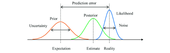
Top-down predictions are not just about the content of lower-level representations but also about our [the brain’s] confidence in those representations (Prediction error in the figure above).
For example, driving on a dark night with rain and fog in a familiar path back home, you put more weight on the prior understanding of the roads than the noisy and untrustworthy incoming signals from the outside world. On the other hand, driving on an unfamiliar road in the day you put more weight on the bottom-up stream of data (likelihood) than the priors (generative model).
Relation to Machine learning
In prediction-driven learning, the world can be relied upon to provide a training signal allowing us to compare current predictions with actual sensed patterns of energetic input. This allows well-understood learning algorithms to unearth rich information about the interacting external causes (‘latent variables’) that are actually structuring the incoming signal. But in practice, this requires an additional and vital ingredient. That ingredient is the use of multilevel learning.
Prediction-driven learning operating in hierarchical (multilayer) settings plausibly holds the key to learning about our kind of world: a world that is highly structured, displaying regularity and pattern at many spatial and temporal scales, and populated by a wide variety of interacting and complexly nested distal causes.
In machine learning, such insights helped inspire a cascade of crucial innovations beginning with work on the aptly named ‘Helmholtz Machine’. The Helmholtz Machine was an early example of a multilayer architecture trainable without reliance upon experimenter pre-classified examples. Instead, the system ‘self-organized’ by attempting to generate the training data for itself, using its own downwards (and lateral) connections. That is to say, instead of starting with the task of classifying (or ‘learning a recognition model for’) the data, it had first to learn how to generate, using a multilevel system, the incoming data for itself.
But before knowing more about that we first should understand the simpler model which is the Restricted Boltzmann Machine (RBM). It is consists of one hidden layer that can represent the latent variables and a visible layer that can represent the sensory inputs in the PP framework. The connections between visible and hidden variables are undirected. Also, the weights on them start with random numbers. Given any input data, the weight can be used to calculate the values on hidden nodes. But the interesting part is that the hidden nodes also can reconstruct the visible nodes. Of course, using initial random weight the construction would be wrong but using an algorithm known as contrastive divergence we can learn the proper weight.
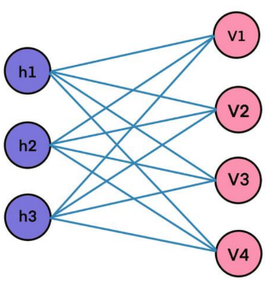
There are actually two modes for an RBM. The flow from visible nodes to hidden nodes (resembles the bottom-up in PP) and from hidden nodes to visible nodes for reconstruction (resembles the top-down in PP). This analogy is not perfect in any way because we don’t calculate any errors or precision weighting but the fact that such a model can go through a phase know as “daydreaming” shows that it has so many similarities with the top-down flow of the brain that in some ways “reconstruct” the reality!
In this demo you can create inputs and let the network train and then ask the model to do the daydreaming, what happens is that the network starts to recreate almost the same inputs as output. Here I tried to force the network to remember and reconstruct only one pattern and when the daydreaming starts it can reconstruct it.
In contrast, A Helmholtz machine contains two networks, a bottom-up recognition network that takes the data as input and produces a distribution over hidden variables, and a top-down “generative” network that generates values of the hidden variables and the data itself.
Helmholtz machines are trained by using the so-called ‘wake-sleep’ algorithm where the wake and sleep phases are not contrastive. Rather, the recognition and generative models are forced to chase the other.

In this way, Helmholtz machines resemble the PP framework more than RBM’s.
References:
[1] Clark, Andy. Surfing uncertainty: Prediction, action, and the embodied mind. Oxford University Press, 2015.
[3] https://matthewho.me/restricted-boltzmann-machine-visualizer/
[4] Yanagisawa, Hideyoshi, Oto Kawamata, and Kazutaka Ueda. “Modeling emotions associated with novelty at variable uncertainty levels: A Bayesian approach.” Frontiers in computational neuroscience 13 (2019): 2.